Transformations
We can now put shapes on the screen, colour them per vertex and wrap textures around them. They just sit there, though. To make something move we could rewrite its vertices every frame and upload the buffer again, but that is slow, and the buffers in our lessons are immutable anyway: the GPU got them once, at creation, and the CPU never touches them again. The usual answer, and the one every chapter from here on relies on, is to leave the vertices alone and hand the vertex shader a
Matrices are one of those subjects that look forbidding until you have used them a few times, after which they become an everyday tool. This chapter is the maths groundwork for the rest of the tutorial: vectors first, then matrices, then how the two combine into transformations. If some of it does not stick on the first read, that is normal; skim it, carry on, and come back when a later chapter leans on it. At the end we put it to work with math.asm, the small library that does for our lessons what GLM does for LearnOpenGL.
Vectors
A
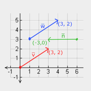
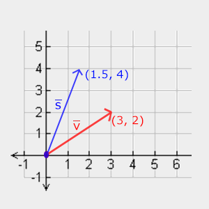
Because a vector is only a direction and a length, it has no fixed starting point. In LearnOpenGL's picture below, \(\color{red}{\bar{v}}\) and \(\color{blue}{\bar{w}}\) start in different places but are the same vector, (3, 2): three to the right, two up.
On paper a vector is written as a letter with a bar, \(\bar{v}\), and its components are stacked in a column:
\[\bar{v} = \begin{pmatrix} \color{red}x \\ \color{green}y \\ \color{blue}z \end{pmatrix}\]
We also use vectors for positions. The trick is to fix the start of the vector at the origin, (0, 0, 0): the vector then points at exactly one spot, and that spot is the position. The vertex positions we have been writing into buffers are vectors read this way, and so are the colours and texture coordinates, which are just "a few numbers that belong together". In math.asm they are plain structures of 32-bit floats:
vec3 struct
    x real4 ?
    y real4 ?
    z real4 ?
vec3 ends
with vec2 and vec4 alongside, so z_axis vec3 <0.0, 0.0, 1.0> in a lesson's data is the unit z direction. In HLSL the same things are called float2, float3 and float4, which we have been using since the first triangle.
Scalar vector operations
A
Multiplication is the one we use most: it keeps the direction and changes the length. math.asm calls it
Vector negation
Negating a vector flips it around: same length, opposite direction. Every component gets a minus sign, which is the same as scaling by -1:
\[-\bar{v} = -\begin{pmatrix} \color{red}{v_x} \\ \color{green}{v_y} \\ \color{blue}{v_z} \end{pmatrix} = \begin{pmatrix} -\color{red}{v_x} \\ -\color{green}{v_y} \\ -\color{blue}{v_z} \end{pmatrix}\]Addition and subtraction
Two vectors are added component by component:
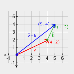
\[\bar{v} = \begin{pmatrix} \color{red}4 \\ \color{green}2 \\ \color{blue}0 \end{pmatrix}, \bar{k} = \begin{pmatrix} \color{red}1 \\ \color{green}2 \\ \color{blue}0 \end{pmatrix} \rightarrow \bar{v} + \bar{k} = \begin{pmatrix} \color{red}{4 + 1} \\ \color{green}{2 + 2} \\ \color{blue}{0 + 0} \end{pmatrix} = \begin{pmatrix} \color{red}5 \\ \color{green}4 \\ \color{blue}0 \end{pmatrix}\]Drawn as arrows, addition means walking the first vector and then the second from where the first ended. The sum is the arrow from the very start to the very end:
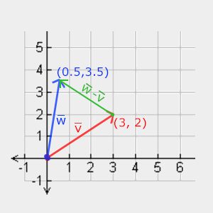
Subtraction is adding the negated vector. Its useful property is geometric: \(\bar{w} - \bar{v}\) is the vector that leads from the point \(\bar{v}\) to the point \(\bar{w}\). Whenever we need "the direction from here to there", from a surface to a light or from the camera to its target, it is a subtraction of two positions.
Length
The components of a 2D vector are the two short sides of a right-angled triangle, and the vector itself is the long side:
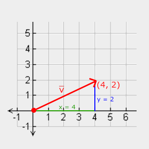
So Pythagoras gives its length, written \(||\bar{v}||\), and in 3D we simply add the third square:
\[||\bar{v}|| = \sqrt{{\color{red}x}^2 + {\color{green}y}^2 + {\color{blue}z}^2}, \qquad ||(4, 2, 0)|| = \sqrt{16 + 4 + 0} = \sqrt{20} \approx 4.47\]
A vector of length exactly 1 is a
Unit vectors are what we use whenever only the direction matters, as it will for surface normals and light directions. In math.asm:
; rcx: a -> xmm0: |a|
align 16
v3_length proc
    v3load xmm0, [rcx]
    dpps xmm0, xmm0, 71h
    sqrtss xmm0, xmm0
    ret
v3_length endp

; rcx: out, rdx: a. A zero vector stays zero.
align 16
v3_normalize proc
    v3load xmm0, [rdx]
    movaps xmm1, xmm0
    dpps xmm1, xmm1, 7Fh        ; |a|^2 in every lane
    xorps xmm2, xmm2
    comiss xmm1, xmm2
    je done
    sqrtps xmm1, xmm1
    divps xmm0, xmm1
    done:
    v3store [rcx], xmm0
    ret
v3_normalize endp
The length is computed through the dot product, which is coming next (dpps), and a zero vector, which has no direction to keep, is handed back unchanged rather than divided by zero.
xmm register holds four floats, called ps ("packed single") works on all four at once, where one ending in ss ("scalar single") works on the lowest lane only. math.asm that move a vec3's twelve bytes into lanes x, y and z of a register, with 0 in the fourth, and back. So divps divides x, y and z by the length in one instruction. The procedures take vectors and matrices by address, in the usual rcx, rdx, r8, and write their results through an out address; a float result comes back in xmm0.
Vector-vector multiplication
There is no single obvious way to multiply two vectors. Multiplying them component by component exists (HLSL's * on two float3s does that, and mulps), and we will use it for colours, but geometrically the two products that matter are the
Dot product
The dot product of two vectors is a single number: their two lengths multiplied together, times the cosine of the angle \(\theta\) between them.
\[\bar{v} \cdot \bar{k} = ||\bar{v}|| \cdot ||\bar{k}|| \cdot \cos \theta\]
For unit vectors both lengths are 1 and the formula collapses to \(\hat{v} \cdot \hat{k} = \cos \theta\). That is what makes it so handy. The cosine is 1 when the vectors point the same way, 0 when they are at right angles (
Computing it is cheap: multiply matching components and add the results. Two unit vectors in the xy plane, for example:
\[\begin{pmatrix} \color{red}{0.6} \\ \color{green}{0.8} \\ \color{blue}0 \end{pmatrix} \cdot \begin{pmatrix} \color{red}{0.8} \\ \color{green}{0.6} \\ \color{blue}0 \end{pmatrix} = ({\color{red}{0.6 \cdot 0.8}}) + ({\color{green}{0.8 \cdot 0.6}}) + ({\color{blue}{0 \cdot 0}}) = 0.96\]
and the inverse cosine, \(\cos^{-1}(0.96)\), says they are about 16.3 degrees apart. For vectors that are not unit length we would first divide by both lengths. SSE4.1 has the dot product as one instruction, dpps, so ours is short:
; rcx: a, rdx: b -> xmm0: a . b
align 16
v3_dot proc
    v3load xmm0, [rcx]
    v3load xmm1, [rdx]
    dpps xmm0, xmm1, 71h        ; multiply x, y, z; sum into lane 0
    ret
v3_dot endp
The 71h is a mask: its high four bits (7) choose which lanes are multiplied, x, y and z, and its low four (1) which lanes receive the sum, only the first, which is where a float result belongs. 7Fh to get the sum in every lane, ready to divide all three components by.
HLSL has it built in as
Cross product
The cross product only exists in three dimensions. It takes two vectors that are not parallel and returns a third that is perpendicular to both. If the two inputs are already perpendicular to each other, the three together form a set of axes, which is exactly how we will build the camera's frame in a later chapter.
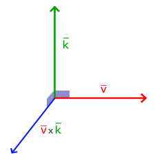
The formula has no obvious picture behind it without some linear algebra, so it is fine to treat it as a recipe:
\[\begin{pmatrix} \color{red}{A_x} \\ \color{green}{A_y} \\ \color{blue}{A_z} \end{pmatrix} \times \begin{pmatrix} \color{red}{B_x} \\ \color{green}{B_y} \\ \color{blue}{B_z} \end{pmatrix} = \begin{pmatrix} \color{green}{A_y} \color{blue}{B_z} - \color{blue}{A_z} \color{green}{B_y} \\ \color{blue}{A_z} \color{red}{B_x} - \color{red}{A_x} \color{blue}{B_z} \\ \color{red}{A_x} \color{green}{B_y} - \color{green}{A_y} \color{red}{B_x} \end{pmatrix}\]; rcx: out, rdx: a, r8: b. (a.y b.z - a.z b.y, a.z b.x - a.x b.z, a.x b.y - a.y b.x)
align 16
v3_cross proc
v3load xmm0, [rdx]
v3load xmm1, [r8]
movaps xmm2, xmm0
movaps xmm3, xmm1
shufps xmm0, xmm0, 0C9h ; a.yzx
shufps xmm1, xmm1, 0D2h ; b.zxy
mulps xmm0, xmm1
shufps xmm2, xmm2, 0D2h ; a.zxy
shufps xmm3, xmm3, 0C9h ; b.yzx
mulps xmm2, xmm3
subps xmm0, xmm2
v3store [rcx], xmm0
ret
v3_cross endp
The formula's left-hand products all pair a component of \(A\) with a different one of \(B\), in a rotating pattern, and so do the right-hand ones. shufps reorders the lanes of a register, so two shuffles line up \((A_y, A_z, A_x)\) against \((B_z, B_x, B_y)\), one mulps makes all three left-hand products, two more shuffles and a mulps make the right-hand ones, and a subps finishes all three components together.
Try it on the x and y axes: \((1, 0, 0) \times (0, 1, 0) = (0, 0, 1)\), the z axis. The order matters: \(\bar{B} \times \bar{A}\) points the opposite way. Which way "x cross y" points is what makes a coordinate system right-handed, and ours is: +x to the right, +y up, +z out of the screen towards us. We come back to that in Coordinate Systems.
Matrices
A
Element (2, 3), second row and third column, is 5. Note the order: row first, the opposite of the (x, y) habit from graphs. Matrices themselves are nothing more than this grid. What makes them interesting is a handful of operations defined on them.
Addition and subtraction
Two matrices of the same size are added or subtracted element by element, each with its counterpart in the same row and column. Matrices of different sizes cannot be added at all.
\[\begin{bmatrix} \color{red}3 & \color{red}1 \\ \color{green}0 & \color{green}5 \end{bmatrix} + \begin{bmatrix} \color{red}2 & \color{red}2 \\ \color{green}4 & \color{green}1 \end{bmatrix} = \begin{bmatrix} \color{red}5 & \color{red}3 \\ \color{green}4 & \color{green}6 \end{bmatrix}, \qquad \begin{bmatrix} \color{red}3 & \color{red}1 \\ \color{green}0 & \color{green}5 \end{bmatrix} - \begin{bmatrix} \color{red}2 & \color{red}2 \\ \color{green}4 & \color{green}1 \end{bmatrix} = \begin{bmatrix} \color{red}1 & -\color{red}1 \\ -\color{green}4 & \color{green}4 \end{bmatrix}\]Matrix-scalar products
Multiplying a matrix by a scalar multiplies every element by it, which is where the word "scalar" comes from: it scales everything by the same amount.
\[{\color{green}3} \cdot \begin{bmatrix} 1 & 0 \\ 2 & 4 \end{bmatrix} = \begin{bmatrix} 3 & 0 \\ 6 & 12 \end{bmatrix}\]Matrix-matrix multiplication
Multiplying two matrices is the operation everything else depends on, and the one that takes a little practice. Two rules come first:
- The left matrix must have as many columns as the right matrix has rows. Otherwise the product is not defined.
- The order matters: in general \(A \cdot B \neq B \cdot A\). Multiplication of matrices is not commutative.
Each element of the result pairs one row of the left matrix with one column of the right matrix. Walk along the row and down the column together, multiply the pairs of numbers you meet, and add them up. The row you used is the row of the result element, and the column you used is its column. LearnOpenGL's diagram colours the pairings:

Written out:
\[\begin{bmatrix} \color{red}1 & \color{red}2 \\ \color{green}3 & \color{green}4 \end{bmatrix} \cdot \begin{bmatrix} \color{blue}5 & \color{purple}6 \\ \color{blue}7 & \color{purple}8 \end{bmatrix} = \begin{bmatrix} \color{red}1 \cdot \color{blue}5 + \color{red}2 \cdot \color{blue}7 & \color{red}1 \cdot \color{purple}6 + \color{red}2 \cdot \color{purple}8 \\ \color{green}3 \cdot \color{blue}5 + \color{green}4 \cdot \color{blue}7 & \color{green}3 \cdot \color{purple}6 + \color{green}4 \cdot \color{purple}8 \end{bmatrix} = \begin{bmatrix} 19 & 22 \\ 43 & 50 \end{bmatrix}\]The result has as many rows as the left matrix and as many columns as the right one. Every element is a dot product, of a row with a column, which is one more reason the dot product keeps turning up. Here is the same thing for 4x4 matrices, the only size our lessons use, in the form SSE likes best:
; rcx: out, rdx: a, r8: b -> out = a * b
;
; Row i of the product is a[i][0] * b.row0 + a[i][1] * b.row1 + a[i][2] * b.row2 + a[i][3] * b.row3.
; b is read into registers first and each row of a is read before its row of out is written, so
; out may be a or b.
align 16
m4_mul proc
    movups xmm2, [r8]
    movups xmm3, [r8 + 16]
    movups xmm4, [r8 + 32]
    movups xmm5, [r8 + 48]
    for row, <0, 16, 32, 48>
        movss xmm0, dword ptr [rdx + row]
        splat xmm0
        mulps xmm0, xmm2
        movss xmm1, dword ptr [rdx + row + 4]
        splat xmm1
        mulps xmm1, xmm3
        addps xmm0, xmm1
        movss xmm1, dword ptr [rdx + row + 8]
        splat xmm1
        mulps xmm1, xmm4
        addps xmm0, xmm1
        movss xmm1, dword ptr [rdx + row + 12]
        splat xmm1
        mulps xmm1, xmm5
        addps xmm0, xmm1
        movups [rcx + row], xmm0
    endm
    ret
m4_mul endp
It is the same sum, grouped differently. Rather than one dot product per element, it builds a whole row of the result at once: row \(i\) of the product is row 0 of b times \(a_{i0}\), plus row 1 of b times \(a_{i1}\), and so on, which you can check against the formula above. Each row of b is four floats, one movups into one register, and mulps. The for ... endm is not a loop at run time: it is MASM's repeat block, which writes its body out four times, with row standing for 0, 16, 32 and 48, the byte offsets of the four rows. Doing a couple of products by hand is still the fastest way to make the pattern stick; after that, let the computer do it.
Matrix-vector multiplication
A vector with N components is really an Nx1 matrix: N rows, one column. So a matrix with N columns can multiply it, and the result is another vector. That is the whole point of this chapter. A great many useful operations, moving, turning, stretching, and later projecting, can be packed into a matrix, and multiplying a vector by that matrix applies the operation to it.
Identity matrix
The plainest 4x4 matrix is the
Each result element is a row of the matrix dotted with the vector, and each row has a single 1 that picks out one component. A transformation that does nothing sounds pointless, but it is where every other transformation starts: take the identity and change a few elements.
; rcx: out
align 16
m4_identity proc
    xorps xmm0, xmm0
    movups [rcx], xmm0
    movups [rcx + 16], xmm0
    movups [rcx + 32], xmm0
    movups [rcx + 48], xmm0
    mov eax, 3F800000h          ; 1.0
    mov [rcx + 0], eax
    mov [rcx + 20], eax
    mov [rcx + 40], eax
    mov [rcx + 60], eax
    ret
m4_identity endp
Four 16-byte stores of zero clear the matrix, and then the diagonal gets 1.0, written by its bits, 3F800000h. Elements 0, 5, 10 and 15 are the diagonal, at byte offsets 0, 20, 40 and 60, because a mat4 keeps its 16 floats in m, row after row: element (row, column) is m[row * 4 + col], four bytes each. We will see why that matters once the matrix travels to a shader.
Scaling
The identity matrix already multiplies each component by the 1 on its row. Replace those ones with other factors and each component is multiplied by those instead:
\[\begin{bmatrix} \color{red}{S_x} & \color{red}0 & \color{red}0 & \color{red}0 \\ \color{green}0 & \color{green}{S_y} & \color{green}0 & \color{green}0 \\ \color{blue}0 & \color{blue}0 & \color{blue}{S_z} & \color{blue}0 \\ \color{purple}0 & \color{purple}0 & \color{purple}0 & \color{purple}1 \end{bmatrix} \cdot \begin{pmatrix} x \\ y \\ z \\ 1 \end{pmatrix} = \begin{pmatrix} \color{red}{S_x} \cdot x \\ \color{green}{S_y} \cdot y \\ \color{blue}{S_z} \cdot z \\ 1 \end{pmatrix}\]; rcx: out, rdx: s (vec3) -> a scale by s
align 16
m4_scale proc
mov r8, rdx
call m4_identity
mov eax, [r8].vec3.x
mov [rcx + 0], eax
mov eax, [r8].vec3.y
mov [rcx + 20], eax
mov eax, [r8].vec3.z
mov [rcx + 40], eax
ret
m4_scale endp
It starts from the identity, by calling out, still in rcx. That works because we wrote xmm0, eax and memory; the scale vector's address is moved to r8 first all the same, since rdx is not ours to keep across a call. The factors are copied as four-byte patterns through eax: moving a float needs no floating-point instruction.
The fourth diagonal element stays 1. The fourth component of the vector, w, has a job of its own, which the next transformation explains.
Translation
; rcx: out, rdx: t (vec3) -> a translation by t
align 16
m4_translate proc
    mov r8, rdx
    call m4_identity
    mov eax, [r8].vec3.x
    mov [rcx + 12], eax
    mov eax, [r8].vec3.y
    mov [rcx + 28], eax
    mov eax, [r8].vec3.z
    mov [rcx + 44], eax
    ret
m4_translate endp
Elements 3, 7 and 11, at byte offsets 12, 28 and 44, are the last column of rows 0, 1 and 2, exactly where the formula puts \(T_x\), \(T_y\) and \(T_z\).
Rotation
Rotations take a little trigonometry. An angle can be measured in degrees, 360 to a full turn, or in math.asm work in radians, so we convert with
; xmm0: degrees -> xmm0: radians
align 16
radians proc
    mulss xmm0, math_degrees_to_radians
    ret
radians endp
A quarter turn is 90 degrees, or \(\pi/2\) radians; a fifth of a turn is 72 degrees, as between \(\bar{k}\) and \(\bar{v}\) here:
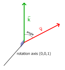
In 3D a rotation is an angle plus an
To rotate about some other axis you could chain these, x then y then z, but chained axis rotations suffer from
Set the axis to (0, 0, 1) and it reduces to \(R_z\) above.
; rcx: out, xmm1: angle in radians, r8: axis (vec3)
;
; A rotation of `angle` about `axis`, counter-clockwise when looking down the axis towards the
; origin.
align 16
m4_rotate proc out_ref:qword, angle:qword, axis_ref:qword
    local a:vec3, c:real4, s:real4, t:real4

    movss real4 ptr angle, xmm1 ; the prologue homed rdx here, not xmm1
    lea rcx, a
    mov rdx, axis_ref
    call v3_normalize
    movss xmm0, real4 ptr angle
    call cosf
    movss c, xmm0
    movss xmm1, math_one
    subss xmm1, xmm0
    movss t, xmm1
    movss xmm0, real4 ptr angle
    call sinf
    movss s, xmm0

    mov rcx, out_ref
    call m4_identity
    ; r.m[0] = c + a.x * a.x * t
    movss xmm0, a.x
    mulss xmm0, a.x
    mulss xmm0, t
    addss xmm0, c
    movss real4 ptr [rcx + 0], xmm0
    ; r.m[1] = a.x * a.y * t - a.z * s
    movss xmm0, a.x
    mulss xmm0, a.y
    mulss xmm0, t
    movss xmm1, a.z
    mulss xmm1, s
    subss xmm0, xmm1
    movss real4 ptr [rcx + 4], xmm0
    ; ...
    ret
m4_rotate endp
The formula needs a unit axis, so the function normalizes whatever it is given, into the local a.
Look at where the angle arrives. It is the second argument, so by the Win64 rule it comes in xmm1, the xmm register of the second position, even though the first argument, out, is an integer in rcx. Each argument position owns one integer and one xmm register, and an argument uses whichever suits its type. MASM's proc doesn't know which arguments are floats, and the prologue stores rdx into the angle's slot on the stack, as it would for any second argument, so the procedure's first instruction overwrites that slot with xmm1, and from then on angle means the float. Then the cosine and sine come from math.asm's fcos and fsin instructions: there is no C library to call.
Even this form can be driven into gimbal lock if the angles come from three separate Euler angles; the cure for that is
Combining matrices
Here is the real reason to use matrices: several transformations multiply together into one matrix, and that single matrix then does all of them at once, for every vertex, for the price of one. Suppose we want to halve a shape's size and then move it by (2, 1, 0). The translation matrix times the scale matrix is:
\[T \cdot S = \begin{bmatrix} \color{red}1 & \color{red}0 & \color{red}0 & \color{red}2 \\ \color{green}0 & \color{green}1 & \color{green}0 & \color{green}1 \\ \color{blue}0 & \color{blue}0 & \color{blue}1 & \color{blue}0 \\ \color{purple}0 & \color{purple}0 & \color{purple}0 & \color{purple}1 \end{bmatrix} \cdot \begin{bmatrix} \color{red}{0.5} & \color{red}0 & \color{red}0 & \color{red}0 \\ \color{green}0 & \color{green}{0.5} & \color{green}0 & \color{green}0 \\ \color{blue}0 & \color{blue}0 & \color{blue}{0.5} & \color{blue}0 \\ \color{purple}0 & \color{purple}0 & \color{purple}0 & \color{purple}1 \end{bmatrix} = \begin{bmatrix} \color{red}{0.5} & \color{red}0 & \color{red}0 & \color{red}2 \\ \color{green}0 & \color{green}{0.5} & \color{green}0 & \color{green}1 \\ \color{blue}0 & \color{blue}0 & \color{blue}{0.5} & \color{blue}0 \\ \color{purple}0 & \color{purple}0 & \color{purple}0 & \color{purple}1 \end{bmatrix}\]and applied to a position:
\[\begin{bmatrix} \color{red}{0.5} & \color{red}0 & \color{red}0 & \color{red}2 \\ \color{green}0 & \color{green}{0.5} & \color{green}0 & \color{green}1 \\ \color{blue}0 & \color{blue}0 & \color{blue}{0.5} & \color{blue}0 \\ \color{purple}0 & \color{purple}0 & \color{purple}0 & \color{purple}1 \end{bmatrix} \cdot \begin{pmatrix} x \\ y \\ z \\ 1 \end{pmatrix} = \begin{pmatrix} \color{red}{0.5x + 2} \\ \color{green}{0.5y + 1} \\ \color{blue}{0.5z} \\ 1 \end{pmatrix}\]Halved, then moved, as we wanted. Notice which way round that is. In \(T \cdot S \cdot \bar{v}\) the matrix nearest the vector, \(S\), touches it first, so a product of transformations is read right to left. Multiply them the other way, \(S \cdot T\), and the translation happens first and then gets halved along with everything else: the shape lands at (1, 0.5, 0) instead. Because of this, the usual order is scale first, then rotate, then translate, which in a product reads \(T \cdot R \cdot S\): scaling and rotating then happen around the shape's own centre, before it is moved away from the origin.
In practice
Neither Direct3D nor HLSL gives the CPU side any vector or matrix types, so the program needs its own. LearnOpenGL uses GLM. The usual choice for Direct3D in C++ is Microsoft's DirectXMath, but it is a C++ library built around SIMD types, and it treats vectors as rows, multiplying \(\bar{v} \cdot M\), so every product in LearnOpenGL would have to be written the other way round. Our lessons instead use includes/math.asm, SSE procedures that keep LearnOpenGL's conventions, as its opening comment says:
;   * right-handed world: +x right, +y up, the camera looks down -z
;   * column vectors: a point is transformed as `M * p`, so `T * R * S` scales first and
;     translates last
;   * clip-space depth runs 0..1, which is D3D's range (GL's is -1..1)
The first and last points belong to the next two chapters. The second is what we just worked through: a matrix times a column vector, read right to left. Everything in this chapter is a procedure in math.asm. Where GLM writes a + b we call A * B is invoke m4_mul, ADDR result, ADDR A, ADDR B.
One difference from GLM is worth knowing before reading LearnOpenGL's code side by side with ours. GLM's glm::translate(trans, v) takes an existing matrix and returns it multiplied by a translation, so LearnOpenGL builds a transformation in steps:
glm::mat4 trans = glm::mat4(1.0f);
trans = glm::translate(trans, glm::vec3(0.5f, -0.5f, 0.0f));
trans = glm::rotate(trans, (float)glfwGetTime(), glm::vec3(0.0f, 0.0f, 1.0f));
Our
; rcx: out, rdx: m, r8: v -> out = m * v
align 16
m4_mul_v4 proc
    movups xmm4, [r8]
    movups xmm0, [rdx]
    mulps xmm0, xmm4
    movups xmm1, [rdx + 16]
    mulps xmm1, xmm4
    movups xmm2, [rdx + 32]
    mulps xmm2, xmm4
    movups xmm3, [rdx + 48]
    mulps xmm3, xmm4
    haddps xmm0, xmm1           ; row sums, two lanes at a time
    haddps xmm2, xmm3
    haddps xmm0, xmm2
    movups [rcx], xmm0
    ret
m4_mul_v4 endp
(2, 1, 0), with w still 1. haddps, which adds neighbouring lanes, sum the four rows' products into one register, a component in each lane.
Getting the matrix to the shader
The vertex shader needs the matrix, and per-draw values reach shaders through a constant buffer, as the tint did in Shaders. HLSL's matrix type is float4x4, and
// Read matrices row by row, as rin stores them; mul(M, v) is then M * v.
#pragma pack_matrix(row_major)

cbuffer object : register(b0)
{
    float4x4 transform;
};
...
vs_out vs_main(float3 position : POSITION, float2 uv : TEXCOORD)
{
    vs_out o;
    o.position = mul(transform, float4(position, 1.0));
    o.uv = uv;
    return o;
}
The position arrives as a float3 and we give it a w of 1 before multiplying, since it is a point that should be translated. The result is what the shader returns as SV_Position, so the rasterizer sees the moved square. The pixel shader is unchanged from Textures: the crate with 20% of the face mixed in.
The first line, the #pragma, is the one Direct3D detail in this chapter, and forgetting it is a classic. A mat4 is 16 floats, and the CPU and the shader have to agree on what order they are in. We store them row by row, as we saw with math.asm stores them the same way.) HLSL, by default, expects a matrix in a constant buffer to be stored column by column (#pragma pack_matrix(row_major) tells the compiler our matrices are mul(transform, v) means exactly \(M \cdot \bar{v}\), as in our maths and as transform * v does in GLSL.
mul(v, M) in Direct3D code elsewhere: that treats the vector as a row and expects matrices built the transposed way, the DirectXMath convention. We never use that form.
On the CPU side, a structure mirrors the constant buffer:
object_constants struct
    transform mat4 <>
object_constants ends
A mat4 is 64 bytes, four of HLSL's 16-byte registers, so the buffer's size is already a multiple of 16 as constant buffers require. The buffer is made once with b0 every frame with invoke bind_constants, 0, constants, which binds it for the vertex, geometry and pixel stages alike:
; rcx: register (b0, b1, ...), rdx: buffer
;
; The same buffer in the same register for the vertex, geometry and pixel stages.
align 16
bind_constants proc slot:qword, buffer:qword
    vcall context, ID3D11DeviceContext_VSSetConstantBuffers, slot, 1, ADDR buffer
    vcall context, ID3D11DeviceContext_GSSetConstantBuffers, slot, 1, ADDR buffer
    vcall context, ID3D11DeviceContext_PSSetConstantBuffers, slot, 1, ADDR buffer
    ret
bind_constants endp
ADDR buffer works because the prologue stored the argument in its stack slot: the methods want an array of buffers, and that slot is an array of one.
Putting it together
The lesson draws the textured square twice, from the same vertex and index buffers, each time with its own matrix. Because the matrices change with time, they are rebuilt every frame inside the render loop. The matrices and vectors are globals in the data section: translation, rotation, scale_ and aspect are mat4s, bottom_right, top_left and z_axis are vec3 constants such as bottom_right vec3 <0.5, -0.5, 0.0>, and c is the object_constants that is copied into the buffer:
; transform = aspect * translate(0.5, -0.5, 0) * rotate(time, z)
invoke m4_translate, ADDR translation, ADDR bottom_right
lea rcx, rotation
movss xmm1, current_frame
lea r8, z_axis
call m4_rotate
invoke m4_mul, ADDR c.transform, ADDR translation, ADDR rotation
invoke m4_mul, ADDR c.transform, ADDR aspect, ADDR c.transform
invoke update_buffer, constants, ADDR c, sizeof object_constants
vcall context, ID3D11DeviceContext_DrawIndexed, 6, 0, 0

; transform = aspect * translate(-0.5, 0.5, 0) * scale(|sin(time)|)
movss xmm0, current_frame
call sinf
andps xmm0, math_abs_mask
movss pulse.x, xmm0
movss pulse.y, xmm0
movss pulse.z, xmm0
invoke m4_translate, ADDR translation, ADDR top_left
invoke m4_scale, ADDR scale_, ADDR pulse
invoke m4_mul, ADDR c.transform, ADDR translation, ADDR scale_
invoke m4_mul, ADDR c.transform, ADDR aspect, ADDR c.transform
invoke update_buffer, constants, ADDR c, sizeof object_constants
vcall context, ID3D11DeviceContext_DrawIndexed, 6, 0, 0
xmm1, which rcx, xmm1 and r8, and the procedure is simply called. Since andps with math_abs_mask clears the sign bit of every lane.
Read each one from the right. The first square is rotated about z by current_frame radians, the seconds since start, so it turns about once every six seconds; only then is it translated to the bottom right. It spins in place, around its own centre, because it is rotated while that centre is still at the origin. The second square is scaled by \(|\sin t|\), shrinking to nothing and growing back, and then moved to the top left. LearnOpenGL leaves that second square as an exercise; our lesson draws both. The absolute value keeps the scale positive; a plain sine would also work but would flip the square through itself every other cycle.
Between the two draws we write the constant buffer again.
Then there is aspect, applied last, after everything else. LearnOpenGL does not have it:
; aspect = scale(height / width, 1, 1)
cvtsi2ss xmm1, scr_height
cvtsi2ss xmm0, scr_width
divss xmm1, xmm0
movss pulse.x, xmm1
storef pulse.y, 1.0
storef pulse.z, 1.0
invoke m4_scale, ADDR aspect, ADDR pulse
It doesn't change, so it is made once, before the render loop, borrowing the pulse vector to hold the scale factors.
Clip space runs from -1 to 1 in both x and y, but our window is 1280 by 720 pixels, so one unit of x covers more pixels than one unit of y. Scaling x by 720/1280 makes a unit the same size on screen in both directions, and the squares stay square while they spin. Because it is the leftmost matrix, it also squeezes the translations: the first square's centre ends up at x = 0.28 rather than 0.5. In the next chapter a projection matrix takes over this job.
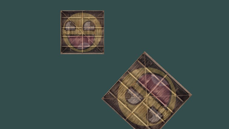
That is two moving objects without touching a single vertex. A matrix can hold as many transformations as we like, and the vertex shader applies them all with one multiplication; all the CPU uploads each frame is 64 bytes. The full program is here, its shaders here, and the maths library here.
Next we use matrices to set up several coordinate spaces, and take the step into 3D.
Additional resources
- Essence of Linear Algebra: Grant Sanderson's video series, the clearest visual explanation of what matrices do.
- Matrix Multiplication: an interactive animation of rows meeting columns.
- Per-component math operations: Microsoft's notes on HLSL matrices,
mul, and row- and column-major packing. - LearnOpenGL's Transformations: the OpenGL version of this chapter, with GLM.
Exercises
- Swap the order of the first square's matrices so it is translated first and rotated second. Work out on paper what should happen before you run it, then check.
- Delete
#pragma pack_matrix(row_major)fromtransformations.hlsland run the lesson. Explain what you see in terms of the transposed matrix, then put the pragma back and get the same broken picture by passing the matrix throughm4_transpose (rcxthe result,rdxthe matrix, which may be the same) beforeupdate_buffer . - Add a third square in the top right that both spins and pulses. Mind the order of the scale and the rotation (does it matter here?) and of the translation.